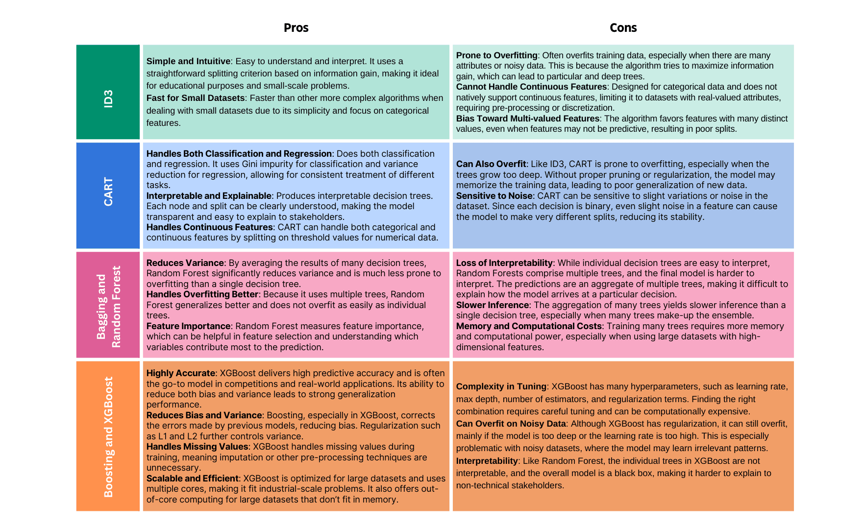
Random Forest vs XGBoost: Speed & Accuracy on California Housing

Benchmark two popular tree ensemble regressors—Random Forest and XGBoost—on the California Housing dataset, comparing accuracy and timing.

Estimated reading time: ~18 minutes

Overview

Random Forest and XGBoost are widely used ensemble methods for tabular regression. This article compares their performance on the California Housing dataset using default-ish settings (100 trees) and reports:

• Predictive accuracy (MSE, R²)
• Training and prediction wall-clock times
• Error dispersion via predicted vs actual plots with ±1 standard deviation bands

All code is included for reference only (non-executable here). Figures are pre-rendered by a headless script scripts/generate_rf_xgb_figures.py.

1. Imports & dataset

import numpy as np
import time
from sklearn.datasets import fetch_california_housing
from sklearn.model_selection import train_test_split
from sklearn.ensemble import RandomForestRegressor
from xgboost import XGBRegressor
from sklearn.metrics import mean_squared_error, r2_score

data = fetch_california_housing()
X, y = data.data, data.target
X_train, X_test, y_train, y_test = train_test_split(
    X, y, test_size=0.2, random_state=42
)
X.shape  # (n_observations, n_features)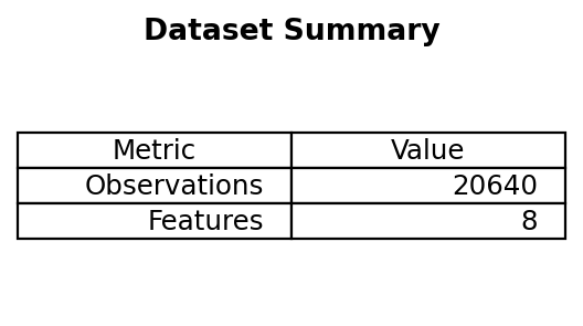

Dataset summary

2. Model initialization

n_estimators = 100
rf = RandomForestRegressor(n_estimators=n_estimators, random_state=42)
xgb = XGBRegressor(n_estimators=n_estimators, random_state=42, verbosity=0)

3. Training & timing

start = time.time(); rf.fit(X_train, y_train); rf_train_time = time.time() - start
start = time.time(); xgb.fit(X_train, y_train); xgb_train_time = time.time() - start

4. Prediction & timing

start = time.time(); y_pred_rf = rf.predict(X_test); rf_pred_time = time.time() - start
start = time.time(); y_pred_xgb = xgb.predict(X_test); xgb_pred_time = time.time() - start

5. Metrics

mse_rf = mean_squared_error(y_test, y_pred_rf)
mse_xgb = mean_squared_error(y_test, y_pred_xgb)
r2_rf = r2_score(y_test, y_pred_rf)
r2_xgb = r2_score(y_test, y_pred_xgb)
summary = {
    'Random Forest': {'MSE': mse_rf, 'R2': r2_rf, 'train_s': rf_train_time, 'pred_s': rf_pred_time},
    'XGBoost': {'MSE': mse_xgb, 'R2': r2_xgb, 'train_s': xgb_train_time, 'pred_s': xgb_pred_time}
}
summary

Performance summary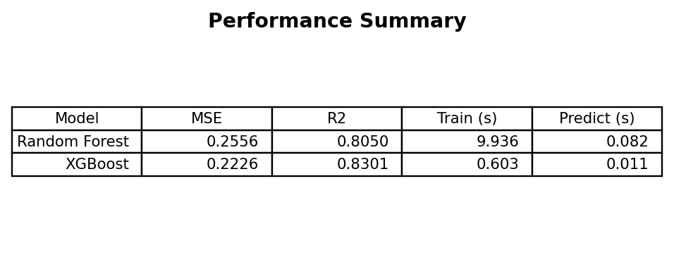

Quick interpretation

• XGBoost often yields slightly better MSE/R² with faster prediction (and sometimes faster training depending on hardware and parameters).
• Random Forest is competitive and can be simpler to tune initially.

6. Predicted vs actual dispersion

std_y = np.std(y_test)
# (Plotting code would create side-by-side scatter charts with ideal & ±1σ bands.)

Predicted vs actual (±1σ bands)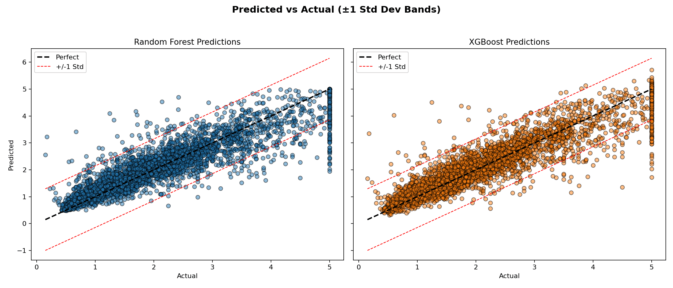

Observations

• Most residuals lie within ±1 std dev of the target for both models.
• Random Forest tends to under-shoot extremes; XGBoost may overshoot upper tail values.
• Heteroscedasticity is mild; variance remains fairly stable across target range.

7. When to choose which?

Scenario	Prefer Random Forest	Prefer XGBoost
Baseline prototype	✅ Simple start	—
Highly tuned leaderboard pursuit	—	✅ Usually superior
Small data, low variance need	✅ Robust	✅ (with regularization)
Need calibrated feature importance (averaging)	✅	Mixed (gain-based)
Tight latency constraints	Sometimes	✅ Often faster

8. Next improvement ideas

• Hyperparameter tuning: depth, learning rate (XGBoost), min child weight, subsampling.
• Feature engineering & interaction creation.
• Cross-validation with early stopping for XGBoost.
• Shapley value analysis for interpretability.
• Consider LightGBM or CatBoost for alternative gradient boosting variants.

9. Key takeaways

• Both models perform strongly out-of-the-box on structured regression.
• XGBoost typically edges ahead in accuracy/time trade-off due to gradient boosting optimizations.
• Random Forest remains a solid, low-friction baseline and a robustness benchmark.
• Visualization of residual structure complements scalar metrics.